Data modeling
June 21, 2018
Often it happens to have a stochastic process producing Independent Identically Distributed (IID) variables one has to interpret. Let \(\mathbf{X}\) be our (continuous or discrete) random variable and \(x_1,\dots,x_n \in \mathbb{R}\) a random sample we got from it.
One important step for data interpretation is trying to generalize the samples and build a model of the stochastic variable distribution generating it. In this way we can predict future outcomes \(x_{n+1},x_{n+2}\dots\) or design systems dealing with the underlying stochastic process.
In these notes are listed few techniques to build distribution models out of sample data; the first technique class distinction is between:
- techniques guessing the model;
- techniques without model guess (a.k.a., parameter-free).
Model guessing techniques include moment method and Maximum Likelihood Estimation (MLE). The other class includes Kernel Density Estimation (KDE).
\[\newcommand{\openopt}{\begin{align}} \newcommand{\closeopt}{\end{align}}\]Model guessing
The first and most simple techniques require to guess a distribution model among the most famous ones (Normal, Gamma, Weibull, etc..) and compute its parameters from the estimated moments.
Let’s say we receive this IID sample: \(x = 2.22559726e+00, 1.38605086e+00, 5.16310220e-01, 7.63338546e-01,9.82043622e-02, 7.26430609e-01, 1.36663134e-01, 7.79299107e-01,1.53225070e-04, 2.42064909e+00, 1.57446991e-01, 1.37291131e+00, 8.28241661e-02, 9.30933968e-02, 1.73380834e+00, 1.80158675e-02, 3.74066727e-01, 1.97124991e+00, 2.32550182e-02, 5.45637333e-03\)
In python we can plot the frequency histogram to grasp ideas:
import matplotlib.pyplot as plt

x = [2.22559726e+00, 1.38605086e+00, 5.16310220e-01, 7.63338546e-01,9.82043622e-02, 7.26430609e-01, 1.36663134e-01, 7.79299107e-01,1.53225070e-04, 2.42064909e+00, 1.57446991e-01, 1.37291131e+00, 8.28241661e-02, 9.30933968e-02, 1.73380834e+00, 1.80158675e-02,  3.74066727e-01, 1.97124991e+00, 2.32550182e-02, 5.45637333e-03]

plt.hist(x, normed=True)
plt.xlabel("Value")
plt.ylabel("Frequency")
plt.show()
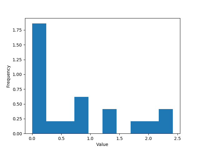
With the experienced data analyst eye we can guess data could be generated by an exponential process.
Spoiler it was not, never trust your eyes, it comes from a gamma distribution.
Moment method
Exponential distributions have one parameter, \(\lambda\), that completely characterizes them. So if we can compute the \(\lambda\) parameter for the (supposed) exponential distribution that generated our data \(X\) we are done.
Considering the exponential moments, we note that \(E[X] = \frac{1}{\lambda}\)
We do not know the expected value of \(X\) but, luckily, we have a good estimator for it, the mean. \(\mu = \frac{1}{n}\sum_{i=1}^{n} x_i\)
So, we can compute \(\lambda = \frac{1}{\mu} = 1.34\)
Note: in Scipy Python library, the distribution function takes the scale parameter \(\beta = \frac{1}{\lambda}\) as input.
import numpy as np
import scipy.stats as stats
z = np.linspace(0, 2.5, 1000)
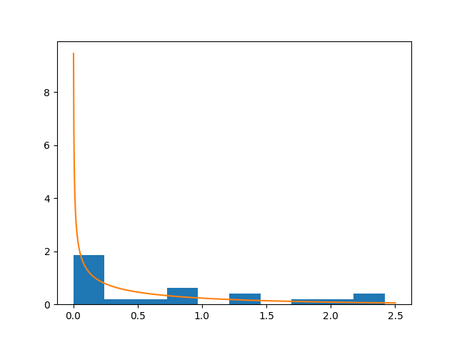
plt.hist(x, normed=True)
plt.plot(z, stats.expon.pdf(z, scale=1/1.34))
plt.show()
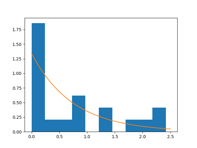
From the figure, our exponential model tries to correctly fit the data and, for some applications, it could be good enough. Anyway, we can try again with the gamma distribution. First we note that the gamma distribution is completely characterized by two parameters: the scale \(\theta\) and the shape \(k\).
We then take into consideration the system composed of gamma first two moments:
\[E[X] = k\theta\\ Var(X) = {k\theta^2}\]The we compute the estimators \(\mu=0.74,\ s^2=\frac{1}{n-1}\sum_i^n(\mu-x_i)^2 = 0.66\); so the system yields: \(\theta = \frac{s^2}{\mu} = 0.89 \\ k = \frac{\mu}{\theta} = 0.83\)
plt.hist(x, normed=True)
plt.plot(z, stats.gamma.pdf(z, 0.83 ,scale=0.89))
plt.show()
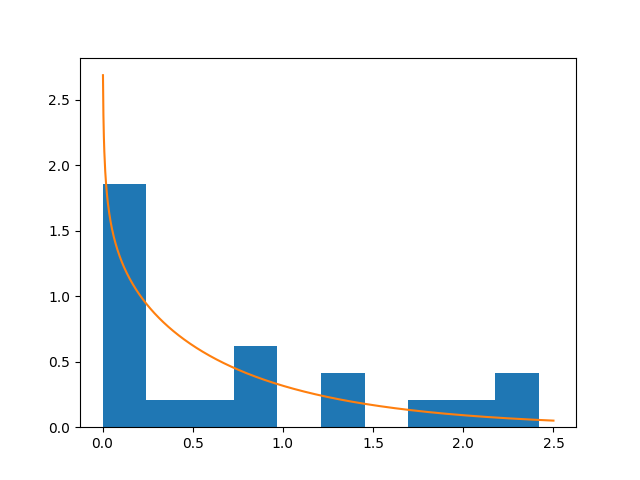
…which captures better the data.
Maximum Likelihood Estimation (MLE)
MLE assumes we identified the right distribution model (the gamma distribution) and we just need to fine tune the parameters (\(k,\theta\)). Instead of relying on the moments, we can consider the Likelikhood \(L(k,\theta)\).
We first consider the likelihood of a single sample \(x_i\), \(L_i(k, \theta) = \frac{x_i^{k-1}e^{-\frac{x_i}{\theta}}}{\Gamma(k)\theta^k}\); which is the value of the gamma probability distribution function for the realization \(x_i\). Then, the likelihood of our whole sample is:
\[L(k,\theta) = \prod_i^n \frac{x_i^{k-1}e^{-\frac{x_i}{\theta}}}{\Gamma(k)\theta^k}\]and it expresses how likely is our sample to come from a gamma distribution with parameters \(k,\theta\) (i.e., \(P(x_1,\dots,x_n \| k,\theta)\)).
To find \(k,\theta\) we now maximize the function \(L(k,\theta)\). Since it includes a product of small numbers and, hence, it is not numerically neat, we prefer to work with its logarithmic counterpart which has the maxima for the same values. \(l(k,\theta) = \log L(k,\theta) = \sum_i^n \log \frac{x_i^{k-1}e^{-\frac{x_i}{\theta}}}{\Gamma(k)\theta^k} = \sum_i^n (k-1) \log x_i - \frac{x_i}{\theta} -\log \Gamma(k) -k\log \theta\)
We need to compute the derivatives of \(l(k,\theta)\) with respect to both \(k, \theta\) and then finding their values for the derivatives equal to zero. Most of the time this computation cannot be done in closed form and we require a numerical method.
We are gonna use Python Scipy optimization function; it targets the minimum value, so we are changing the sign to the log-likelihood function seek its maximum. We also need a starting point and we pick \((0.5,0.5)\) just because it looks nice. We enforce that \(k,\theta>0\) by giving bounding boxes, note that for numerical stability reasons, the minimum is set to \(1^{-10}\).
import scipy.optimization as opt
import scipy.special as sp
import math

def loglikelihood(args):
	# args is a tuple containing k and theta
	k = args[0]
	t = args[1]
	s = 0

	for xi in x:
		s += (k-1)*math.log(xi)
		s -= xi/t
		s -= math.log(sp.gamma(k))
		s -= k*math.log(t)


	return -s

res = opt.minimize(loglikelihood, [0.5, 0.5], bounds=[(1e-10,None),(1e-10,None)])
k,t = res.x  # 0.49, 1.51
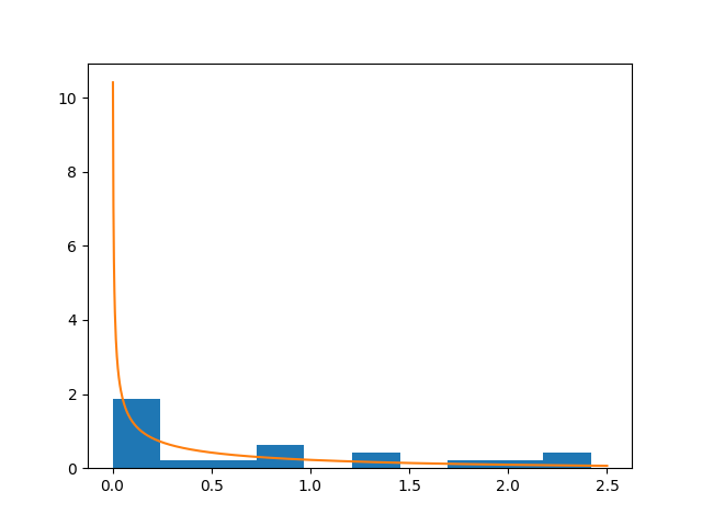
And finally, we can see the result (not extraordinary):
plt.hist(x, normed=True)
plt.plot(z, stats.gamma.pdf(z, k ,scale=t))
plt.show()
Note, however, that Python Scipy ships a function for fitting a gamma distribution to a data sample:
k,l,t = stats.gamma.fit(x)  # 0.44, 0.0, 2.01
plt.hist(x, normed=True)
plt.plot(z, stats.gamma.pdf(z, k ,scale=t))
plt.show()
Conclusions
So, it is time to say the real parameters used to generate the data were: \(k=0.5,\theta=1\).
| Ranking | Name | \(k\) | \(\theta\) |
|---|---|---|---|
| 1 | MLE | 0.49 | 1.51 |
| 2 | Python MLE | 0.44 | 2.01 |
| 3 | Mom. method | 0.83 | 0.89 |
The fact the moment method is failing so bad is probably to the limited sample size which affects the estimation of \(E[X],Var(X)\).
Parameter-free modeling
Kernel density estimation
Histograms are nice and directly built from the samples, their bias consists just in the choice of the binning step. Once normalized, they could be used as probability density functions, however they are discontinuous. Besides being disadvantageous, discontinuity is unlikely for natural phenomena. We can use different structures in place of the bins to represents frequencies and smooth away the discontinuities. That is the intuition behind the kernel density estimation.
A kernel is a non-negative function that integrates to one, \(k():\mathbb{R}\to \mathbb{R}^+\). Popular choices of kernels include: triangle, normal. Kernels have actually one parameter \(h\), called the bandwidth. \(h\) dictates the degree of the smoothing.
The approximated density function becomes:
\[\hat{f}_h(x) = \frac{1}{hn}\sum_i^n k(\frac{x-x_i}{h})\]A magic value for \(h\) when using the normal kernels is \(h^\dagger= (\frac{4s^5}{3n})^{\frac{1}{5}}=0.47\), where \(s\) is the empirical standard deviation.
Using the normal kernels then:
\[\hat{f}(x) = \frac{1}{h^\dagger n} \sum_i^n \frac{1}{\sqrt{2\pi}} e^{-\frac{(x-x_i)^2}{2(h^\dagger)^2}}\]Which is a mixture of Gaussians, one for each sample element \(x_i\), centered at it. Next we are gonna compare our implementation with the one provided by Python Scipy:
n = 20
h = 0.47
def my_pdf(y):
     res = []
     for yi in y:
         s = 0
         for xi in x:
             s += (math.e**(-(yi-xi)**2/(2*h**2)))/math.sqrt(2*math.pi)
         s /= h*n
         res.append(s)
     return res

y = my_pdf(z)
kde = stats.kde.gaussian_kde(x)

plt.hist(x, normed=True)
plt.plot(z, y, label='My KDE')

plt.plot(z, kde(z), label='Python KDE')

plt.legend()
plt.show()
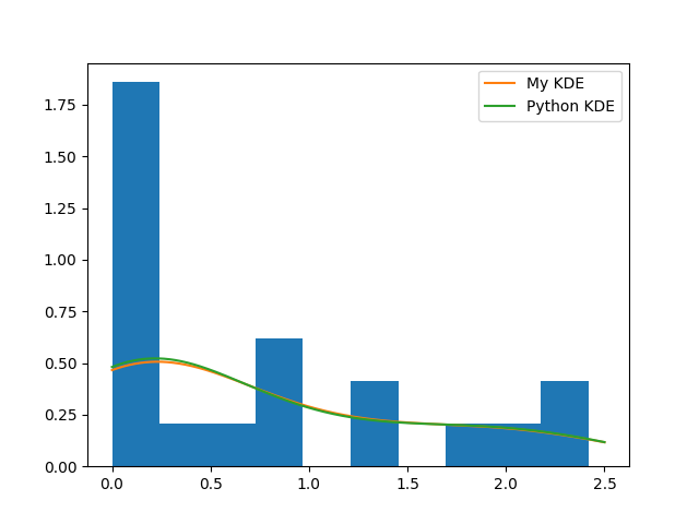
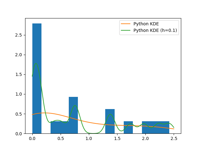
…and both methods really perform badly. Reasons rely on the fact that the original generating model (gamma distribution) is not a mixture of Gaussians and on the computation of the bandwidth parameter \(h\). In fact:
plt.hist(x, bins=15, normed=True)
plt.plot(z, y, label='My KDE (h=0.1)')

plt.plot(z, kde(z), label='Python KDE')
plt.legend()
plt.show()