Wireless communication and Inphase/Quadrature complex samples
February 18, 2022
The most prominent abstraction for wireless communication my group has been using at the Institute for the Wireless Internet-of-Things, is the I/Q samples. These notes collect and summarize information on Inphase/Quadrature for the newcomers to Software Defined Radios and research in wireless communication.
I/Q samples uniquely characterize a waveform (subject to the limitation of the sampling rate frequency) and are used by hardware to convert sampled digital data to waveforms and vice-versa. Modern technologies deal only with digital data, as it is more robust to noise and allows further processing (error detection and correction, encryption, and interpolation).
I/Q samples are so tied to waveforms that I am recalling the latter first, and present their inter-connection to the former.
The Electromagnetic wave
Electromagnetic waves propagate in the space at the speed of light. They are generated by a magnetic field with non zero acceleration.
A continuous electric current (moving charges) generates a static magnetic field. If the direction of moving charges is periodically inverted, the resulting magnetic field is also being inverted, and the transition time of this inversion characterizes the acceleration of the magnetic field.
The easiest electromagnetic wave transmitter to build and understand is probably the spark-gap. Spark-gap works with a circuit which periodically self-stops, generating a kind of series of electromagnetic impulses. It can be useful to send morse-code and it was used at the dawn of wireless communication.
Nowadays, wireless devices use an oscillator. Oscillators are electronic components which produce alternate currents, meaning the resulting magnetic field is oscillating as well (hence having a continuous acceleration). Oscillators produce these alternate currents by generating a voltage whose intensity and orientation follows a sinusoid. As a consequence, the produced electromagnetic field varies as a sinusoid.
Hence, sinusoids are the fundamental functions in wireless communication. Sinusoids are indicated with the functions \(\sin(t),\cos(t)\) (note, \(cos(t)=sin(t+\frac{\pi}{2})\)).
The electromagnetic wave propagates in free space and it induces a magnetic field in a receiver hardware. Hence, the receiver apparatus is ultimately measuring voltage values; these values can be digitalized (sampled) to be processed by micro-processors. In the following, I call \(m(t)\) the voltage readings of a waveform for both the transmitter and the receiver.
The pipeline
The pipeline is the set of transforming steps that takes our digital bits, process them, and uses an electromagnetic sinusoid to transmit them.
Generally a (transmission) pipeline comprises the following:
- Encoding
- Modulation
- Uplink conversion
The encoding step takes our bits as input and produces other bits in output. Its purpose is to make the information contained in the bits more robust against transmission errors. Example of encoding techniques are: Hamming coding and Cyclic Redundancy Coding (CRC).
Modulation takes the bits in output from the previous step and produces in output sinusoid parameters, for each bit (or group of bits) we indicate a particular sinusoid parameter alteration which is embedding that information.
Uplink conversion is about taking the incoming sinusoid parameters and combining them with the oscillator output to create a radio frequency signal.
Modulation
Suppose that we are generating an electromagnetic sinusoid with operating frequency \(F_0\). Our emitted waveform is going to be:
\[m(t) = cos(2\pi F_0t)\]Typically, time is divided in discreet time slots of duration \(\tau\). Provided that the transmitter and the receiver are synchronized on the time slot starting times (a problem solved, but outside of the scope of this article), they use the sinusoid variation to encode bits of information.
Before clarifying with an example, let’s analyse how the sinusoid can be varied. We can modulate (encode) information in a sinusoid in primarily three ways:
- by a change of sinusoid Amplitude (AM)
- by a change of sinusoid Frequency (FM)
- by a change of sinusoid Phase (PM)
The image below shows an example of AM on a sinusoid; the top chart shows the digital data transmitted, the lower chart shows the resulting waveform (for the given operating frequency and modulation settings), and the lower orange bar shows the \(\tau\) intervals.
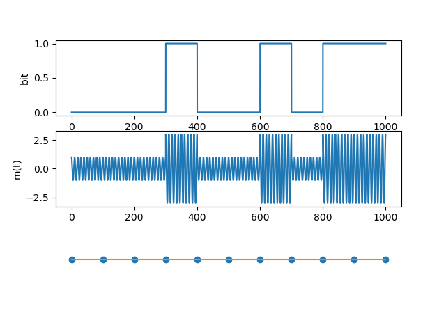
In this case the demodulation consists in the reconstruction of the digital data by comparing the receiving power (amplitude) of the received signal.
Inphase/Quadrature
Inphase/Quadrature coding is an elegant trick to abstract modulation from the actual physical waveform generation circuitry. Instead of building a specific circuitry for each kind of modulation and their specific parameters, we can instead rely on generic hardware.
The following signal include all possible modulation variations (\(a(t)\) for the AM, \(\Delta(t)\) for FM, and \(\phi(t)\) for PM).
\[m(t) = a(t)cos(2\pi(F_0+\Delta(t))t + \phi (t))\]We can reinterpret \(m(t)\) with the exponential (knowing the Euler’s formula \(e^{i\psi} = \cos(\psi)+\sin(\psi)\)) and state its complex envelope:
\[\tilde{m}(t) = a(t)e^{j2\pi(F_0+\Delta(t))t+j\phi(t)} = a(t)e^{j2\pi\Delta(t)t+j\phi (t)}e^{j2\pi F_0t}\]The base band signal is the part of \(\tilde{m}(t)\) independent from the operating frequency (hence, retaining all the meaningful information):
\[m^{bb}(t) = a(t)e^{j2\pi\Delta(t)t+j\phi (t)} = a(t)e^{j\gamma (t)} = i(t)+jq(t)\]\(\gamma (t) = \tan^{-1}(\frac{q(t)}{i(t)})\) and \(a(t) = \sqrt{i^2(t)+q^2(t)}\)
The signal we want to transmit is hence: \(m(t) = R\{\tilde{m}(t)\} = R\{m^{bb}(t)e^{j2\pi F_0t}\} =R\{(i(t)+jq(t))e^{j2\pi F_0t}\} = i(t)cos(2\pi F_0t)-q(t)sin(2\pi F_0t)\)
Where \(R\{\}\) indicates the real part. Note for who can be lost at this point: physics does not allow the generation of imaginary waveforms :) .
Then, we use the following hardware circuit to easily embed \(i(t), q(t)\) upon our oscillator output:
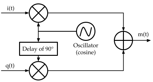
Where we used that \(cos(\psi + \frac{\pi}{2}) = -\sin(\psi)\).
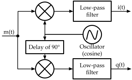
At the receiving side, we get \(m(t)\) from the antenna and the goal is to get \(i(t), q(t)\) back. We note that: \(m(t)\cos(2\pi F_0t) = \frac{i(t)}{2} + i(t)\cos(4\pi F_0t) - \frac{q(t)}{2}\sin(4\pi F_0t)\) and that: \(m(t)\sin(2\pi F_0t) = \frac{q(t)}{2} + \frac{i(t)}{2}\sin(4\pi F_0t) - \frac{1}{2}\sin(4\pi F_0t)\)
Hence, we can get \(i(t),q(t)\) from \(m(t)\) buy multiplying it with sinusoids of the same frequency and filtering out the part with frequency greater than zero.
An image follows:
Remarks
Modern wireless communication deals with digital signals. In order to transform a waveform to a digital signal, one needs to sample it (\(m(t)\)). Instead of working on the waveform samples, we can use their transformation, the I/Q samples, to enable the modularization of specialized hardware, with a dedicated unit to synthesize waveforms from modulation-agnostic samples. Furthermore, in signal processing I/Q samples have the advantages of giving instant information on the amplitude and frequencies.