Luca Baldesi

Statistics is hard and generally counter-intuitive; these notes regard one of the most interesting tools it can provide, hypothesis testing.

Hypothesis testing

Whenever a researcher attempts a certain claim based on data, some statistics is involved. Hypothesis testing is a theoretical framework for dealing with claims and assign them a certain reliability. Meaning that we not only want to know if data supports a claim but also with which degree of probability. Hypothesis testing is used for answering questions like: is this new medicine really effective curing a certain disease?, is the new high-speed mass transport reducing commuting time?

In this context the claim is called the hypothesis and it is paired (for convenience) with its counterpart, the null hypothesis which simply negates it.

We are playing with the following (boring) toy example:

In the USA, elementary students are found with an average QI of 100. The principal of the Springfield elementary school, Skinner, makes 30 students of his undertake a test and he finds out they have an average QI of 112.5 (with a standard deviation of 15).

Immediately, he calls the superintendent Chalmers to request more funds for his gifted pupils. But is his claim statistically correct?

Z-test

Z-test is one of the hypothesis testing available tests and it is applicable when:

• Samples are IID (Independently, identically distributed);
• The number of samples is large (greater than 30) or the standard deviation \(\sigma\) is known.

In our example, Skinner collected \(n=30\) samples with average \(\bar{X}\) which we consider IID. Since \(n\ge 30\), we do not care if \(\sigma=15\) is the true standard deviation or a sample one (for \(n\lt 30\) we should apply the T-test if \(\sigma\) is a sample standard deviation).

The Central Limit Theorem (CLT) states that:

For \(n\) large enough, the random variable \(\sqrt{n}(\bar{X}-\mu)\) is distributed like a Gaussian \(N(0, \sigma^2)\)

Here, \(\mu\) represents the mean of the distribution generating the samples. Being the normal distribution symmetric, it naturally follows:

which is more straightforward for our purposes (because we are ultimately interested in the random variable \(\mu\)).

Note that the CLT works no matter what distribution generated the samples; the sample average will be always distributed as a Gaussian.

In our example, Skinner is trying to prove that the mean \(\mu\) for QI in Springfield school is not the same as the one for the rest of young kids in the USA. His hypothesis is thus:

• H1: \(\mu\gt 100\)

while, Chalmers (and the hypothesis testing framework) are evaluating the opposite hypothesis:

• H0: \(\mu\le 100\)

In fact, this framework accepts the initial hypothesis by rejecting the null hypothesis (a version of Reductio ad absurdum).

Namely, it is now Chalmers’ job to prove Skinner wrong (and negate further funding). Chalmers picks a certain level of confidence, and claims that he will discard H0 only if it has a probability below \(\alpha=5\%\).

From the CLT equation we obtain that:

\begin{equation} \mu \sim N(\bar{X},\frac{\sigma^2}{n}) \label{eq:mudist} \end{equation} \begin{equation} Z = \frac{\mu-\bar{X}}{\sigma/\sqrt{n}} \sim N(0, 1) \label{eq:zdist} \end{equation}

The first equation gives the probability distribution function for \(\mu\), based on the observed sample data. The latter is the Z that gives the name to the test and represents the standardization of \(\mu\) wrt the normal distribution with mean 0 and variance 1.

The following analysis and test is independent either we work on the \(\mu\) or the \(Z\) random variable. I think the former is more intuitive and the latter a residual of pre-computer era where people used to search in precomputed tables the values needed instead of interacting with a computer. I present both approaches as the Z test is now widely accepted and discussed.

\(\mu\) statistic

Back to our example, Skinner’s claim is that \(\mu\) is larger than 100 and its probability of being less than 100 is negligible. Chalmers defines this negligibility as 5% of probability.

We call \(p\)-value the probability under H0 to have observed our sample. It represents the likelihood of the sample under H0. In our example, the \(p\)-value is the probability of having \(\mu \le 100\) for our sampled data.

The following image presents the distribution of \(\mu\) (the blue line) given our sample data, its average \(\bar{X}\) and the cut at 100, the real average according to H0. The \(p\)-value is given by the area underlying the blue curve from \(-\inf\) to \(100\).

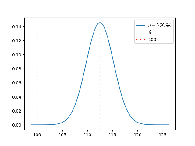
Computing the probability \(p\)-value \(=P\{\mu \le 100\}\) is hence trivial as computing the cumulative distribution function of the first equation, in Python

>>> import scipy.stats as stats
>>> stats.norm(112.5, 2.7386).cdf(100)
2.505e-06

Since \(p\)-value \(=2.505e-06\lt 0.05 = \alpha\) we can reject H0 and declare that H1 holds with a confidence of 95% (and possibly higher, till 1-\(p\)-value). Skinner rejoices!

Z statistic

A more common way to proceed (but equivalent) with this test is using the Z statistic (the standardization of \(\mu\)). We first compute \(Z_0\) as Z under the H0 hypothesis:

>>> (100-112.5)*math.sqrt(30)/15
-4.564354645876384

The image below presents this time the distribution of \(Z\) (i.e., the distribution of the sample average given the observed sample data after standardization) which is nothing but the normal distribution with mean \(0\) and variance \(1\), and the cut point which this time is not directly \(100\), but its standardization, \(Z_0\).

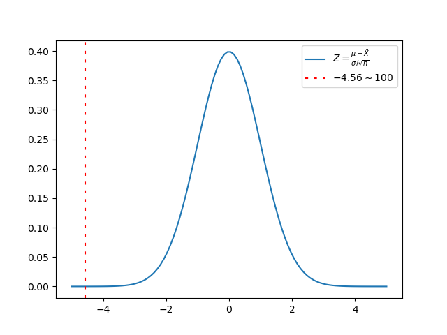
Given \(Z_0=-4.56\) and the \(Z\) distribution function we now hence compute the probability \(P\{Z\le Z_0\}\) which is the area underlying the blue curve in the above image from \(-\inf\) to \(Z_0\).

>> stats.norm(0,1).cdf(-4.56)
2.5051659781952214e-06

Consequently, \(p\)-value \(= 2.505e-06\). Again, since \(p\)-value is less than \(\alpha\) we reject H0 in favor of H1.

T-test

The T-test has been developed to address the limitation of the Z-test regarding the sample size. It still requires the samples to be IID but it can be safely used whatever value of \(n\) we have.

Everything works as in the case of the Z-test, but we focus on the \(T\) statistic instead of the \(Z\) one:

\begin{equation} T = \frac{\mu-\bar{X}}{\sigma/\sqrt{n}} \sim T(n-1) \end{equation}

In fact, \(T\) is still the distribution of the sample average given the observed sample data after standardization, but we know that for sample variance with \(n<30\) it does not distribute anymore like a normal distribution but, instead, like a student distribution (which is also symmetric and bell-shaped).

Here, \(\sigma\) indicates the sample standard deviation and \(T(n-1)\) represents the t-student distribution function with \(n-1\) degrees of freedom.

Again, we can compute the cutting value:

Again, as in the latter case of the Z-test, we compute the p-value:

>>> stats.t(29).cdf(-4.56)
4.3005975438384246e-05

(The interested reader might appreciate that for \(n>>1\) the t-student and Gaussian distributions converge and \(n=30\) has been selected as the threshold at which the two distribution are not significantly different anymore. Hence, we can use the normal distribution and the Z-test with sample variance when \(n\ge 30\)). Which yields to the same comparison, \(p\)-value \(=4.3e-05 \lt \alpha = 0.05\)

Hence, Chalmers has to surrender and recognize Springfield kids result more clever than the average USA student. From here to invest more funding in their education, though, it is all another story.